The usual error analysis of the symmetric eigenproblem (using any LAPACK routine in subsection 2.2.4 or any EISPACK routine) is as follows [64]:
The computed eigendecompositionis nearly the exact eigendecomposition of A + E, i.e.,
is a true eigendecomposition so that
is orthogonal, where
and
. Here p(n) is a modestly growing function of n. We take p(n) = 1 in the above code fragment. Each computed eigenvalue
differs from a true
by at most
Thus large eigenvalues (those near
) are computed to high relative accuracy and small ones may not be.
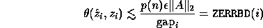
The angular difference between the computed unit eigenvector
and a true unit eigenvector
satisfies the approximate bound
if
is small enough. Here
is the absolute gap between
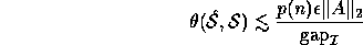
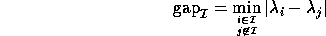
Let
be the invariant subspace spanned by a collection of eigenvectors
, where
is a subset of the integers from 1 to n. Let S be the corresponding true subspace. Then
is the absolute gap between the eigenvalues in
.
In the special case of a real symmetric tridiagonal matrix T, the eigenvalues and eigenvectors can be computed much more accurately. xSYEV (and the other symmetric eigenproblem drivers) computes the eigenvalues and eigenvectors of a dense symmetric matrix by first reducing it to tridiagonal form T, and then finding the eigenvalues and eigenvectors of T. Reduction of a dense matrix to tridiagonal form T can introduce additional errors, so the following bounds for the tridiagonal case do not apply to the dense case.
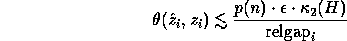
The eigenvalues of T may be computed with small componentwise relative backward error () by using subroutine xSTEBZ (subsection 2.3.4) or driver xSTEVX (subsection 2.2.4). If T is also positive definite, they may also be computed at least as accurately by xPTEQR (subsection 2.3.4). To compute error bounds for the computed eigenvalues
and
. Then the computed eigenvalues
where p(n) is a modestly growing function of n. Thus if
is moderate, each eigenvalue will be computed to high relative accuracy, no matter how tiny it is. The eigenvectors
if
is the relative gap between
Jacobi's method [69][76][24] is another algorithm for finding eigenvalues and eigenvectors of symmetric matrices. It is slower than the algorithms based on first tridiagonalizing the matrix, but is capable of computing more accurate answers in several important cases. Routines implementing Jacobi's method and corresponding error bounds will be available in a future LAPACK release.