
Engineering and Scientific Subroutine Library for AIX Version 3 Release 3: Guide and Reference
These subroutines compute the minimal norm linear least squares solution of
AX is congruent to B, where A is a general
matrix, using the singular value decomposition computed by SGESVF or
DGESVF.
Table 118. Data Types
| V, UB, X, s, tau
| Subroutine
|
| Short-precision real
| SGESVS
|
| Long-precision real
| DGESVS
|
| Fortran
| CALL SGESVS | DGESVS (v, ldv, ub,
ldub, nb, s, x, ldx, m,
n, tau)
|
| C and C++
| sgesvs | dgesvs (v, ldv, ub, ldub,
nb, s, x, ldx, m, n,
tau);
|
| PL/I
| CALL SGESVS | DGESVS (v, ldv, ub,
ldub, nb, s, x, ldx, m,
n, tau);
|
- v
- is the orthogonal matrix V of order n in the singular
value decomposition of matrix A. It is produced by a
preceding call to SGESVF or DGESVF, where it corresponds to output argument
a.
Specified as: an ldv by (at least) n array,
containing numbers of the data type indicated in Table 118.
- ldv
- is the leading dimension of the array specified for v.
Specified as: a fullword integer; ldv > 0 and
ldv >= n.
- ub
- is an n by nb matrix, containing
UTB. It is produced by a preceding
call to SGESVF or DGESVF, where it corresponds to output argument
b. On output, UTB is
overwritten; that is, the original input is not preserved.
Specified as: an ldub by (at least) nb array,
containing numbers of the data type indicated in Table 118.
- ldub
- is the leading dimension of the array specified for ub.
Specified as: a fullword integer; ldub > 0 and
ldub >= n.
- nb
- is the number of columns in matrices X and
UTB. Specified as: a fullword
integer; nb > 0.
- s
- is the vector s of length n, containing the singular
values of matrix A. It is produced by a preceding call to
SGESVF or DGESVF, where it corresponds to output argument s.
Specified as: a one-dimensional array of (at least) length
n, containing numbers of the data type indicated in Table 118;
si >= 0.
- x
- See On Return.
- ldx
- is the leading dimension of the array specified for x.
Specified as: a fullword integer; ldx > 0 and
ldx >= n.
- m
- is the number of rows in matrix A. Specified as: a
fullword integer; m >= 0.
- n
- is the number of columns in matrix A, the order of matrix
V, the number of elements in vector s, the number of
rows in matrix UB, and the number of rows in matrix
X. Specified as: a fullword integer;
n >= 0.
- tau
- is the error tolerance tau. Any singular values in vector
s that are less than tau are treated as zeros when computing matrix
X. Specified as: a number of the data type indicated
in Table 118; tau >= 0. For more information on the
values for tau, see Notes.
- x
- is an n by nb matrix, containing the minimal norm linear
least solutions of AX is congruent to B. The
nb column vectors of X contain minimal norm solution
vectors for nb distinct linear least squares problems.
Returned as: an ldx by (at least) nb array,
containing numbers of the data type indicated in Table 118.
- V, X, s, and
UTB can have no common elements;
otherwise the results are unpredictable.
- In problems involving experimental data, tau should reflect the absolute
accuracy of the matrix elements:
- tau >= max(|DELTAij|)
where DELTAij are the errors in
aij. In problems where the matrix elements
are known exactly or are only affected by roundoff errors:
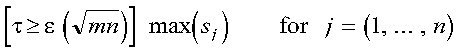
where:
- epsilon is equal to 0.11920E-06 for SGESVS and
0.22204D-15 for DGESVS.
- s is a vector containing the singular values of matrix
A.
For more information, see references [13], [58], [78], and pages
134 to 151 in reference [99].
The minimal norm linear least squares solution of AX is
congruent to B, where A is a real general matrix, is
computed using the singular value decomposition, produced by a preceding call
to SGESVF or DGESVF. From SGESVF or DGESVF, the singular value
decomposition of A is given by the following:
- A = USigmaVT
The linear least squares of solution X, for AX is
congruent to B, is given by the following formula:
- X =
VSigma+UTB
where:
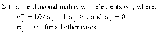
If m or n is equal to 0, no computation is
performed. See references [13], [58], [78],
and pages 134 to 151 in reference [99]. These algorithms have a tendency to generate
underflows that may hurt overall performance. The system default is to
mask underflow, which improves the performance of these subroutines.
None
- ldv <= 0
- n > ldv
- ldub <= 0
- n > ldub
- ldx <= 0
- n > ldx
- nb <= 0
- m < 0
- n < 0
- tau < 0
This example finds the linear least squares solution for the
underdetermined system AX is congruent to B, using the
singular value decomposition computed by DGESVF. Matrix A
is:
                       *               *
                       | 1.0  2.0  2.0 |
                       | 2.0  4.0  5.0 |
                       *               *
and matrix B is:
                           *     *
                           | 1.0 |
                           | 4.0 |
                           *     *
On output, matrix UTB is
overwritten.
- Note:
- This example corresponds to Example 3 of DGESVF on page "Example 3".
             V  LDV  UB  LDUB  NB  S   X  LDX  M   N   TAU
             |   |   |    |    |   |   |   |   |   |    |
CALL DGESVS( V , 3 , UB , 3  , 1 , S , X , 3 , 2 , 3 , TAU )
        *                        *
        | -0.304  -0.894   0.328 |
V    =  | -0.608   0.447   0.656 |
        | -0.733   0.000  -0.680 |
        *                        *
        *        *
        | -4.061 |
UB   =  |  0.000 |
        | -0.714 |
        *        *

S        =  (7.342, 0.000, 0.305)
TAU      =  0.3993D-14
        *        *
        | -0.600 |
X    =  | -1.200 |
        |  2.000 |
        *        *
This example finds the linear least squares solution for the overdetermined
system AX is congruent to B, using the singular value
decomposition computed by DGESVF. Matrix A is:
                          *          *
                          | 1.0  4.0 |
                          | 2.0  5.0 |
                          | 3.0  6.0 |
                          *          *
and where B is:
                          *           *
                          | 7.0  10.0 |
                          | 8.0  11.0 |
                          | 9.0  12.0 |
                          *           *
On output, matrix UTB is
overwritten.
- Note:
- This example corresponds to Example 4 of DGESVF on page "Example 4".
             V  LDV  UB  LDUB  NB  S   X  LDX  M   N   TAU
             |   |   |    |    |   |   |   |   |   |    |
CALL DGESVS( V , 3 , UB , 3  , 2 , S , X , 2 , 3 , 2 , TAU )
        *                *
        |  0.922  -0.386 |
V    =  | -0.386  -0.922 |
        |   .       .    |
        *                *
        *                  *
        |  -1.310   -2.321 |
UB   =  | -13.867  -18.963 |
        |    .        .    |
        *                  *

S        =  (0.773, 9.508)
TAU      =  0.5171D-14
        *                *
X    =  | -1.000  -2.000 |
        |  2.000   3.000 |
        *                *
[ Top of Page | Previous Page | Next Page | Table of Contents | Index ]