Engineering and Scientific Subroutine Library for AIX Version 3 Release 3: Guide and Reference

SAXPY, DAXPY, CAXPY, and ZAXPY--Multiply a Vector X by a Scalar, Add to a Vector Y, and Store in the Vector Y

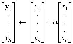
These subprograms perform the following computation, using the scalar alpha and vectors x and y:

y <-- y+alphax

Table 41. Data Types

Syntax

On Entry

n

is the number of elements in vectors x and y. Specified as: a fullword integer; n >= 0.

alpha

is the scalar alpha. Specified as: a number of the data type indicated in Table 41.

x

is the vector x of length n. Specified as: a one-dimensional array of (at least) length 1+(n-1)|incx|, containing numbers of the data type indicated in Table 41.

incx

is the stride for vector x. Specified as: a fullword integer. It can have any value.

y

is the vector y of length n. Specified as: a one-dimensional array of (at least) length 1+(n-1)|incy|, containing numbers of the data type indicated in Table 41.

incy

is the stride for vector y. Specified as: a fullword integer. It can have any value.

On Return

y

is the vector y, containing the results of the computation y+alphax. Returned as: a one-dimensional array, containing numbers of the data type indicated in Table 41.

Notes

1. If you specify the same vector for x and y, incx and incy must be equal; otherwise, results are unpredictable.
2. If you specify different vectors for x and y, they must have no common elements; otherwise, results are unpredictable. See Concepts.

Function

The computation is expressed as follows:

See reference [79]. If alpha or n is zero, no computation is performed. For CAXPY, intermediate results are accumulated in long precision.

Error Conditions

Computational Errors

None

Input-Argument Errors

n < 0

Example 1

This example shows vectors x and y with positive strides.

Call Statement and Input

            N  ALPHA  X  INCX  Y  INCY
            |    |    |   |    |   |
CALL SAXPY( 5 , 2.0 , X , 1  , Y , 2  )
 
X        =  (1.0, 2.0, 3.0, 4.0, 5.0)
Y        =  (1.0, . , 1.0, . , 1.0, . , 1.0, . , 1.0)

Output

Y        =  (3.0, . , 5.0, . , 7.0, . , 9.0, . , 11.0)

Example 2

This example shows vectors x and y having strides of opposite signs. For y, which has negative stride, processing begins at element Y(5), which is 1.0.

Call Statement and Input

            N  ALPHA  X  INCX  Y   INCY
            |    |    |   |    |    |
CALL SAXPY( 5 , 2.0 , X , 1  , Y , -1  )
 
X        =  (1.0, 2.0, 3.0, 4.0, 5.0)
Y        =  (5.0, 4.0, 3.0, 2.0, 1.0)

Output

Y        =  (15.0, 12.0, 9.0, 6.0, 3.0)

Example 3

This example shows a vector, x, with 0 stride. Vector x is treated like a vector of length n, all of whose elements are the same as the single element in x.

Call Statement and Input

            N  ALPHA  X  INCX  Y  INCY
            |    |    |   |    |   |
CALL SAXPY( 5 , 2.0 , X , 0  , Y , 1  )
 
X        =  (1.0)
Y        =  (5.0, 4.0, 3.0, 2.0, 1.0)

Output

Y        =  (7.0, 6.0, 5.0, 4.0, 3.0)

Example 4

This example shows how SAXPY can be used to compute a scalar value. In this case, vectors x and y contain scalar values and the strides for both vectors are 0. The number of elements to be processed, n, is 1.

Call Statement and Input

            N  ALPHA  X  INCX  Y  INCY
            |    |    |   |    |   |
CALL SAXPY( 1 , 2.0 , X , 0  , Y , 0  )
 
X        =  (1.0)
Y        =  (5.0)

Output

Y        =  (7.0)

Example 5

This example shows how to use CAXPY, where vectors x and y contain complex numbers. In this case, vectors x and y have positive strides.

Call Statement and Input

            N  ALPHA  X  INCX  Y  INCY
            |    |    |   |    |   |
CALL CAXPY( 3 ,ALPHA, X , 1  , Y , 2  )
 
ALPHA    =  (2.0, 3.0)
X        =  ((1.0, 2.0), (2.0, 0.0), (3.0, 5.0))
Y        =  ((1.0, 1.0 ), . , (0.0, 2.0), . , (5.0, 4.0))

Output

Y        =  ((-3.0, 8.0), . , (4.0, 8.0), . , (-4.0, 23.0))