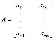

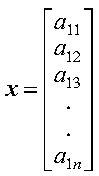
A matrix, also referred to as a general matrix, is an m by n ordered collection of numbers. It is represented symbolically as:
where the matrix is named A and has m rows and n columns. The elements of the matrix are aij, where i = 1, m and j = 1, n.
Matrices can contain either real or complex numbers. Those containing real numbers are called real matrices; those containing complex numbers are called complex matrices.
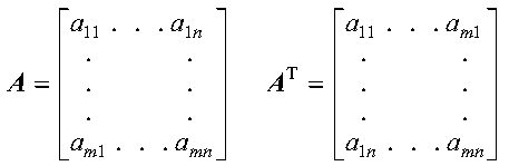
The transpose of a matrix A is a matrix formed from A by interchanging the rows and columns such that row i of matrix A becomes column i of the transposed matrix. The transpose of A is denoted by AT. Each element aij in A becomes element aji in AT. If A is an m by n matrix, then AT is an n by m matrix. The following represents a matrix and its transpose:
ESSL assumes that all matrices are stored in untransformed format, such as matrix A shown above. No movement of data is necessary in your application program when you are processing transposed matrices. The ESSL subroutines adjust their selection of elements from the matrix when an argument in the calling sequence indicates that the transposed matrix is to be used in the computation. Examples of this are the transa and transb arguments specified for SGEADD, matrix addition.
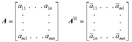
The conjugate transpose of a matrix A, containing complex numbers, is denoted by AH and is expressed as follows:
Just as for the transpose of a matrix, the conjugate transpose of a matrix is stored in untransformed format. No movement of data is necessary in your program.
A matrix is usually stored in a two-dimensional array. Its elements are stored successively within the array. Each column of the matrix is stored successively in the array. The leading dimension argument is used to select the matrix elements from each successive column of the array. The starting point of the matrix in the array is specified as the argument for the matrix in the ESSL calling sequence. For example, if matrix A is contained in array A and starts at the first element in the first row and first column of A, you should specify A as the argument for matrix A, such as in:
CALL SGEMX (5,2,1.0,A,6,X,1,Y,1)
where, in the matrix-vector product, the number of rows in matrix A is 5, the number of columns in matrix A is 2, the scaling constant is 1.0, the location of the matrix is A, the leading dimension is 6, the vectors used in the matrix-vector product are X and Y, and their strides are 1.
If matrix A is contained in the array BIG, declared as BIG(1:20,1:30), and starts at the second row and third column of BIG, you should specify BIG(2,3) as the argument for matrix A, such as in:
CALL SGEMX (5,2,1.0,BIG(2,3),6,X,1,Y,1)
See How Leading Dimension Is Used for Matrices for a complete description of how matrices are stored within arrays.
For a complex matrix, a special storage arrangement is used to accommodate the two parts, a and b, of each complex number (a+bi) in the array. For each complex number, two sequential storage locations are required in the array. Therefore, exactly twice as much storage is required for complex matrices as for real matrices of the same precision. See How Do You Set Up Your Scalar Data? for a description of real and complex numbers, and How Do You Set Up Your Arrays? for a description of how real and complex data is stored in arrays.
The leading dimension for a two-dimensional array is an increment that is used to find the starting point for the matrix elements in each successive column of the array. To define exactly which elements become the conceptual matrix in the array, the following items are used together:
The leading dimension must always be positive. It must always be greater than or equal to m, the number of rows in the matrix to be processed. For an array, A, declared as A(E1:E2,F1:F2), the leading dimension is equal to:
The starting point for selecting the matrix elements from the array is at the location specified by the argument for the matrix in the ESSL calling sequence. For example, if you specify A(3,0) for a 4 by 4 matrix A, where A is declared as A(1:7,0:4):
                 *                             *
                 | 1.0   8.0  15.0  22.0  29.0 |
                 | 2.0   9.0  16.0  23.0  30.0 |
                 | 3.0  10.0  17.0  24.0  31.0 |
                 | 4.0  11.0  18.0  25.0  32.0 |
                 | 5.0  12.0  19.0  26.0  33.0 |
                 | 6.0  13.0  20.0  27.0  34.0 |
                 | 7.0  14.0  21.0  28.0  35.0 |
                 *                             *
then processing begins at the element at row 3 and column 0 in array A, which is 3.0.
The leading dimension is used to find the starting point for the matrix elements in each of the n successive columns in the array. ESSL subroutines assume that the arrays are stored in column-major order, as described under How Do You Set Up Your Arrays?, and they add the leading dimension (times the size of the element in bytes) to the starting point. They do this n-1 times. This finds the starting point in each of the n columns of the array.
In the above example, the leading dimension is:
If the number of columns, n, to be processed is 4, the starting points are: A(3,0), A(3,1), A(3,2), and A(3,3). These are elements 3.0, 10.0, 17.0, and 24.0 for a11, a12, a13, and a14, respectively.
In general terms, this results in the following starting positions of each column in the matrix being calculated as follows:
To find the elements in each column of the array, 1 is added successively to the starting point in the column until m elements are selected. This is why the leading dimension must be greater than or equal to m; otherwise, you go past the end of each dimension of the array. In the above example, if the number of elements, m, to be processed in each column is 4, the following elements are selected from array A for the first column of the matrix: A(3,0), A(4,0), A(5,0), and A(6,0). These are elements 3.0, 4.0, 5.0, and 6.0, corresponding to the matrix elements a11, a21, a31, and a41, respectively.
Column element selection can also be expressed in general terms. Using A(BEGINI,BEGINJ) as the starting point in the array, this results in the following elements being selected from each column in the array:
Combining this with the technique already described for finding the starting point in each column of the array, the resulting matrix in the example is:
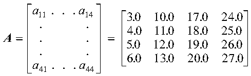
As shown in this example, a matrix does not have to include all columns and rows of an array. The elements of matrix A are selected from rows 3 through 6 and columns 0 through 3 of the array. Rows 1, 2, and 7 and column 4 of the array are not used.
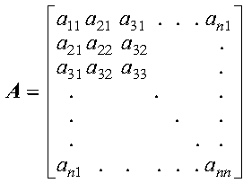
The matrix A is symmetric if it has the property A = AT, which means:
The following matrix illustrates a symmetric matrix of order n; that is, it has n rows and n columns. The subscripts on each side of the diagonal appear the same to show which elements are equal:
The four storage modes used for storing symmetric matrices are described in the following sections:
The storage technique you should use depends on the ESSL subroutine you are using and is given under Notes in each subroutine description.
When a symmetric matrix is stored in lower-packed storage mode, the lower triangular part of the symmetric matrix is stored, including the diagonal, in a one-dimensional array. The lower triangle is packed by columns. (This is equivalent to packing the upper triangle by rows.) The matrix is packed sequentially column by column in n(n+1)/2 elements of a one-dimensional array. To calculate the location of each element aij of matrix A in an array, AP, using the lower triangular packed technique, use the following formula:
This results in the following storage arrangement for the elements of a symmetric matrix A in an array AP:
Following is an example of a symmetric matrix that uses the element values to show the order in which the matrix elements are stored in the array.
Given the following matrix A:
                       *                  *
                       | 1  2   3   4   5 |
                       | 2  6   7   8   9 |
                       | 3  7  10  11  12 |
                       | 4  8  11  13  14 |
                       | 5  9  12  14  15 |
                       *                  *
the array is:
AP = (1, 2, 3, 4, 5, 6, 7, 8, 9, 10, 11, 12, 13, 14, 15)
Following is an example of how to transform your symmetric matrix to lower-packed storage mode:
       K = 0
       DO 1 J=1,N
          DO 2 I=J,N
             K = K+1
             AP(K)=A(I,J)
   2      CONTINUE
   1   CONTINUE
When a symmetric matrix is stored in upper-packed storage mode, the upper triangular part of the symmetric matrix is stored, including the diagonal, in a one-dimensional array. The upper triangle is packed by columns. (This is equivalent to packing the lower triangle by rows.) The matrix is packed sequentially column by column in n(n+1)/2 elements of a one-dimensional array. To calculate the location of each element aij of matrix A in an array AP using the upper triangular packed technique, use the following formula:
This results in the following storage arrangement for the elements of a symmetric matrix A in an array AP:
Following is an example of a symmetric matrix that uses the element values to show the order in which the matrix elements are stored in the array. Given the following matrix A:
                      *                    *
                      |  1   2   4   7  11 |
                      |  2   3   5   8  12 |
                      |  4   5   6   9  13 |
                      |  7   8   9  10  14 |
                      | 11  12  13  14  15 |
                      *                    *
the array is:
AP = (1, 2, 3, 4, 5, 6, 7, 8, 9, 10, 11, 12, 13, 14, 15)
Following is an example of how to transform your symmetric matrix to upper-packed storage mode:
       K = 0
       DO 1 J=1,N
          DO 2 I=1,J
             K = K+1
             AP(K)=A(I,J)
   2      CONTINUE
   1   CONTINUE
When a symmetric matrix is stored in lower storage mode, the lower triangular part of the symmetric matrix is stored, including the diagonal, in a two-dimensional array. These elements are stored in the array in the same way they appear in the matrix. The upper part of the matrix is not required to be stored in the array.
Following is an example of a symmetric matrix A of order 5 and how it is stored in an array AL.
Given the following matrix A:
                       *                  *
                       | 1  2   3   4   5 |
                       | 2  6   7   8   9 |
                       | 3  7  10  11  12 |
                       | 4  8  11  13  14 |
                       | 5  9  12  14  15 |
                       *                  *
the array is:
                       *                  *
                       | 1  *   *   *   * |
                       | 2  6   *   *   * |
                AL  =  | 3  7  10   *   * |
                       | 4  8  11  13   * |
                       | 5  9  12  14  15 |
                       *                  *
where "*" means you do not have to store a value in that position in the array. However, these storage positions are required.
When a symmetric matrix is stored in upper storage mode, the upper triangular part of the symmetric matrix is stored, including the diagonal, in a two-dimensional array. These elements are stored in the array in the same way they appear in the matrix. The lower part of the matrix is not required to be stored in the array.
Following is an example of a symmetric matrix A of order 5 and how it is stored in an array AU.
Given the following matrix A:
                       *                  *
                       | 1  2   3   4   5 |
                       | 2  6   7   8   9 |
                       | 3  7  10  11  12 |
                       | 4  8  11  13  14 |
                       | 5  9  12  14  15 |
                       *                  *
the array is:
                       *                  *
                       | 1  2   3   4   5 |
                       | *  6   7   8   9 |
                 AU =  | *  *  10  11  12 |
                       | *  *   *  13  14 |
                       | *  *   *   *  15 |
                       *                  *
where "*" means you do not have to store a value in that position in the array. However, these storage positions are required.
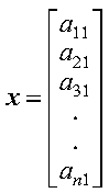
A real symmetric matrix A is positive definite if and only if xTAx is positive for all nonzero vectors x.
A real symmetric matrix A is negative definite if and only if xTAx is negative for all nonzero vectors x.
The positive definite or negative definite symmetric matrix is stored in the same way the symmetric matrix is stored. For a description of this storage technique, see Symmetric Matrix.
A real symmetric matrix A is indefinite if and only if (xTAx) (A yTAy) < 0 for some non-zero vectors x and y.
The symmetric indefinite matrix is stored in the same way the symmetric matrix is stored. For a description of this storage technique, see Symmetric Matrix.
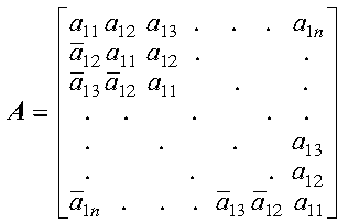
A complex matrix is Hermitian if it is equal to its conjugate transpose:
The complex Hermitian matrix is stored using the same four techniques used for symmetric matrices:
Following is an example of a complex Hermitian matrix H of order 5.
Given the following matrix H:
            *                                              *
            | (11,  0) (21, -1) (31,  1) (41, -1) (51, -1) |
            | (21,  1) (22,  0) (32, -1) (42, -1) (52,  1) |
            | (31, -1) (32,  1) (33,  0) (43, -1) (53, -1) |
            | (41,  1) (42,  1) (43,  1) (44,  0) (54, -1) |
            | (51,  1) (52, -1) (53,  1) (54,  1) (55,  0) |
            *                                              *
it is stored in a one-dimensional array, HP, in n(n+1)/2 = 15 elements as follows:
            HP = ((11, *), (21, 1), (31, -1), (41, 1), (51, 1),
                  (22, *), (32, 1), (42, 1), (52, -1), (33, *),
                  (43, 1), (53, 1), (44, *), (54, 1), (55, *))
            HP = ((11, *), (21, -1), (22, *), (31, 1), (32, -1),
                  (33, *), (41, -1), (42, -1), 43, -1), (44, *),
                  (51, -1), (52, 1), (53, -1), (54, -1), (55, *))
or it is stored in a two-dimensional array, HP, as follows:
          *                                           *
          | (11,  *)   *        *       *       *     |
          | (21,  1) (22,  *)   *       *       *     |
    HP =  | (31, -1) (32,  1) (33, *)   *       *     |
          | (41,  1) (42,  1) (43, 1) (44, *)   *     |
          | (51,  1) (52, -1) (53, 1) (54, 1) (55, *) |
          *                                           *
          *                                             *
          | (11, *) (21, -1) (31,  1) (41, -1) (51, -1) |
          |    *    (22,  *) (32, -1) (42, -1) (52,  1) |
    HP =  |    *       *     (33,  *) (43, -1) (53, -1) |
          |    *       *        *     (44,  *) (54, -1) |
          |    *       *        *        *     (55,  *) |
          *                                             *
where "*" means you do not have to store a value in that position in the array. The imaginary parts of the diagonal elements of a complex Hermitian matrix are always 0, so you do not need to set these values. The ESSL subroutines always assume that the values in these positions are 0.
A complex Hermitian matrix A is positive definite if and only if xHAx is positive for all nonzero vectors x.
A complex Hermitian matrix A is negative definite if and only if xHAx is negative for all nonzero vectors x.
The positive definite or negative definite complex Hermitian matrix is stored in the same way the complex Hermitian matrix is stored. For a description of this storage technique, see Complex Hermitian Matrix.
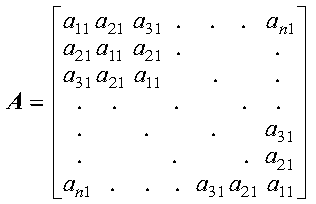
A positive definite or negative definite symmetric matrix A of order n is also a Toeplitz matrix if and only if:
The elements on each diagonal of the Toeplitz matrix have a constant value. For the definition of a positive definite or negative definite symmetric matrix, see Positive Definite or Negative Definite Symmetric Matrix.
The following matrix illustrates a symmetric Toeplitz matrix of order n; that is, it has n rows and n columns:
A symmetric Toeplitz matrix of order n is represented by a vector x of length n containing the elements of the first column of the matrix (or the elements of the first row), such that xi = ai1 for i = 1, n.
The following vector represents the matrix A shown above:
The elements of the vector x, which represent a positive definite symmetric Toeplitz matrix, are stored sequentially in an array. This is called packed-symmetric-Toeplitz storage mode. Following is an example of a positive definite symmetric Toeplitz matrix A and how it is stored in an array X.
Given the following matrix A:
                    *                        *
                    | 99  12  13  14  15  16 |
                    | 12  99  12  13  14  15 |
                    | 13  12  99  12  13  14 |
                    | 14  13  12  99  12  13 |
                    | 15  14  13  12  99  12 |
                    | 16  15  14  13  12  99 |
                    *                        *
the array is:
X = (99, 12, 13, 14, 15, 16)
A positive definite or negative definite complex Hermitian matrix A of order n is also a Toeplitz matrix if and only if:
The real part of the diagonal elements of the Toeplitz matrix must have a constant value. The imaginary part of the diagonal elements must be zero.
For the definition of a positive definite of negative definite complex Hermitian matrix, see Positive Definite or Negative Definite Complex Hermitian Matrix.
The following matrix illustrates a complex Hermitian Toeplitz matrix of order n; that is, it has n rows and n columns:
A complex Hermitian Toeplitz matrix of order n is represented by a vector x of length n containing the elements of the first row of the matrix.
The following vector represents the matrix A shown above.
The elements of the vector x, which represent a positive definite complex Hermitian Toeplitz matrix, are stored sequentially in an array. This is called packed-Hermitian-Toeplitz storage mode. Following is an example of a positive definite complex Hermitian Toeplitz matrix A and how it is stored in an array X.
Given the following matrix A:
     *                                                      *
     |  (10.0, 0.0)   (2.0, -3.0)  (-3.0, 1.0)   (1.0, 1.0) |
     |   (2.0, 3.0)   (10.0, 0.0)  (2.0, -3.0)  (-3.0, 1.0) |
     | (-3.0, -1.0)    (2.0, 3.0)  (10.0, 0.0)  (2.0, -3.0) |
     |  (1.0, -1.0)  (-3.0, -1.0)   (2.0, 3.0)  (10.0, 0.0) |
     *                                                      *
the array is:
X = ((10.0, 0.0), (2.0, -3.0), (-3.0, 1.0), (1.0, 1.0))
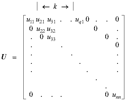
There are two types of triangular matrices: upper triangular matrix and lower triangular matrix. Triangular matrices have the same number of rows as they have columns; that is, they have n rows and n columns.
A matrix U is an upper triangular matrix if its nonzero elements are found only in the upper triangle of the matrix, including the main diagonal; that is:
A matrix L is an lower triangular matrix if its nonzero elements are found only in the lower triangle of the matrix, including the main diagonal; that is:
The following matrices, U and L, illustrate upper and lower triangular matrices of order n, respectively:
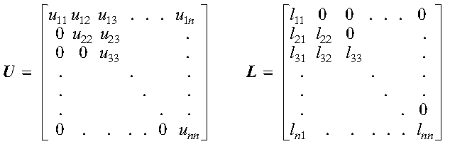
A unit triangular matrix is a triangular matrix in which all the diagonal elements have a value of one; that is:
The following matrices, U and L, illustrate upper and lower unit real triangular matrices of order n, respectively:
The four storage modes used for storing triangular matrices are described in the following sections:
It is important to note that because the diagonal elements of a unit triangular matrix are always one, you do not need to set these values in the array for these four storage modes. ESSL always assumes that the values in these positions are one.
When an upper-triangular matrix is stored in upper-triangular-packed storage mode, the upper triangle of the matrix is stored, including the diagonal, in a one-dimensional array. The upper triangle is packed by columns. The elements are packed sequentially, column by column, in n(n+1)/2 elements of a one-dimensional array. To calculate the location of each element of the triangular matrix in the array, use the technique described in Upper-Packed Storage Mode.
Following is an example of an upper triangular matrix U of order 5 and how it is stored in array UP. It uses the element values to show the order in which the elements are stored in the one-dimensional array.
Given the following matrix U:
                       *                 *
                       | 1  2  4   7  11 |
                       | 0  3  5   8  12 |
                       | 0  0  6   9  13 |
                       | 0  0  0  10  14 |
                       | 0  0  0   0  15 |
                       *                 *
the array is:
UP = (1, 2, 3, 4, 5, 6, 7, 8, 9, 10, 11, 12, 13, 14, 15)
When a lower-triangular matrix is stored in lower-triangular-packed storage mode, the lower triangle of the matrix is stored, including the diagonal, in a one-dimensional array. The lower triangle is packed by columns. The elements are packed sequentially, column by column, in n(n+1)/2 elements of a one-dimensional array. To calculate the location of each element of the triangular matrix in the array, use the technique described in Lower-Packed Storage Mode.
Following is an example of a lower triangular matrix L of order 5 and how it is stored in array LP. It uses the element values to show the order in which the elements are stored in the one-dimensional array.
Given the following matrix L:
                       *                  *
                       | 1  0   0   0   0 |
                       | 2  6   0   0   0 |
                       | 3  7  10   0   0 |
                       | 4  8  11  13   0 |
                       | 5  9  12  14  15 |
                       *                  *
the array is:
LP = (1, 2, 3, 4, 5, 6, 7, 8, 9, 10, 11, 12, 13, 14, 15)
A triangular matrix is stored in upper-triangular storage mode in a two-dimensional array. Only the elements in the upper triangle of the matrix, including the diagonal, are stored in the upper triangle of the array.
Following is an example of an upper triangular matrix U of order 5 and how it is stored in array UTA.
Given the following matrix U:
                      *                    *
                      | 11  12  13  14  15 |
                      |  0  22  23  24  25 |
                      |  0   0  33  34  35 |
                      |  0   0   0  44  45 |
                      |  0   0   0   0  55 |
                      *                    *
the array is:
                      *                    *
                      | 11  12  13  14  15 |
                      |  *  22  23  24  25 |
               UTA =  |  *   *  33  34  35 |
                      |  *   *   *  44  45 |
                      |  *   *   *   *  55 |
                      *                    *
where "*" means you do not have to store a value in that position in the array.
A triangular matrix is stored in lower-triangular storage mode in a two-dimensional array. Only the elements in the lower triangle of the matrix, including the diagonal, are stored in the lower triangle of the array.
Following is an example of a lower triangular matrix L of order 5 and how it is stored in array LTA.
Given the following matrix L:
                      *                    *
                      | 11   0   0   0   0 |
                      | 21  22   0   0   0 |
                      | 31  32  33   0   0 |
                      | 41  42  43  44   0 |
                      | 51  52  53  54  55 |
                      *                    *
the array is:
                      *                    *
                      | 11   *   *   *   * |
                      | 21  22   *   *   * |
                LTA = | 31  32  33   *   * |
                      | 41  42  43  44   * |
                      | 51  52  53  54  55 |
                      *                    *
where "*" means you do not have to store a value in that position in the array.
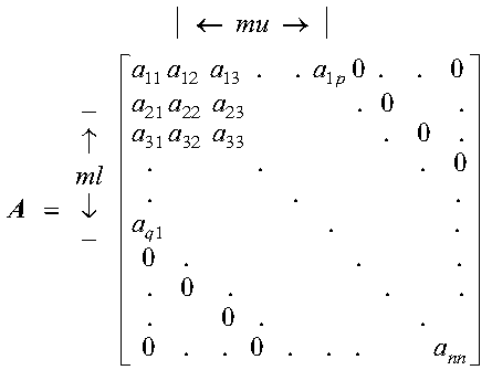
A general band matrix has its nonzero elements arranged uniformly near the diagonal, such that:
where ml and mu are the lower and upper band widths, respectively, and ml+mu+1 is the total band width.
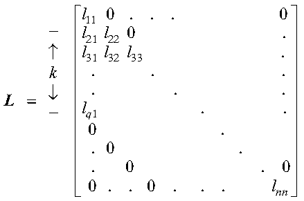
The following matrix illustrates a square general band matrix of order n, where the band widths are ml = q-1 and mu = p-1:
Some special types of band matrices are:
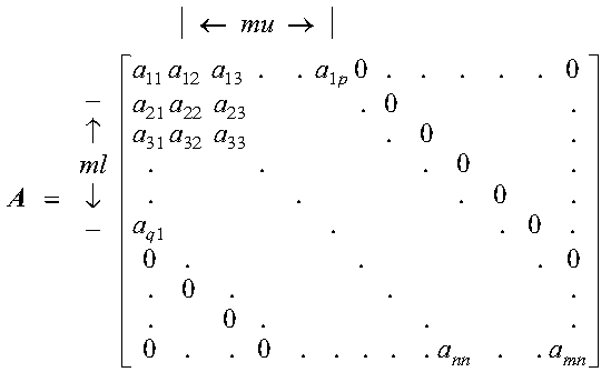
The following two matrices illustrate m by n rectangular general band matrices, where the band widths are ml = q-1 and mu = p-1. For both matrices, the leading diagonal is a11, a22, a33, ..., ann. Following is a general band matrix with m > n:
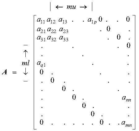
Following is a general band matrix with m < n:
The two storage modes used for storing general band matrices are described in the following sections:
(This storage mode is used only for square matrices.) Only the band elements of a general band matrix are stored for general-band storage mode. Additional storage must also be provided for fill- in. General-band storage mode packs the matrix elements by columns into a two-dimensional array, such that each diagonal of the matrix appears as a row in the packed array.
For a matrix A of order n with band widths ml and mu, the array must have a leading dimension, lda, greater than or equal to 2ml+mu+16. The size of the second dimension must be (at least) n, the number of columns in the matrix.
Using array AGB, which is declared as AGB(2ml+mu+16, n), the columns of elements in matrix A are stored in each column in array AGB as follows, where a11 is stored at AGB(ml+mu+1, 1):
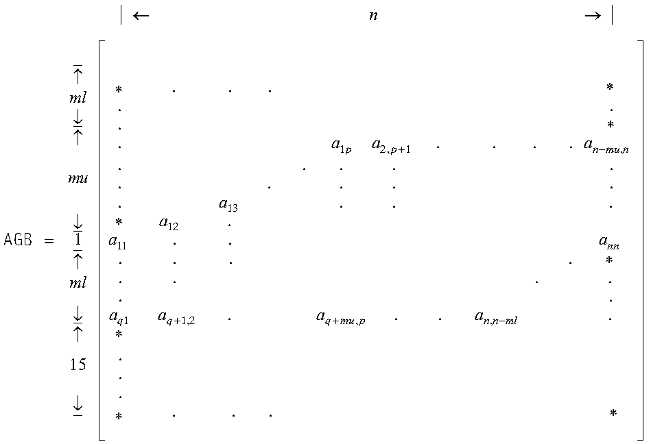
where "*" means you do not store an element in that position in the array.
In the ESSL subroutine computation, some of the positions in the array indicated by an "*" are used for fill- in. Other positions may not be accessed at all.
Following is an example of a band matrix A of order 9 and band widths of ml = 2 and mu = 3.
Given the following matrix A:
              *                                    *
              | 11  12  13  14   0   0   0   0   0 |
              | 21  22  23  24  25   0   0   0   0 |
              | 31  32  33  34  35  36   0   0   0 |
              |  0  42  43  44  45  46  47   0   0 |
              |  0   0  53  54  55  56  57  58   0 |
              |  0   0   0  64  65  66  67  68  69 |
              |  0   0   0   0  75  76  77  78  79 |
              |  0   0   0   0   0  86  87  88  89 |
              |  0   0   0   0   0   0  97  98  99 |
              *                                    *
you store it in general-band storage mode in a 23 by 9 array AGB as follows, where a11 is stored in AGB(6,1):
              *                                    *
              |  *   *   *   *   *   *   *   *   * |
              |  *   *   *   *   *   *   *   *   * |
              |  *   *   *  14  25  36  47  58  69 |
              |  *   *  13  24  35  46  57  68  79 |
              |  *  12  23  34  45  56  67  78  89 |
              | 11  22  33  44  55  66  77  88  99 |
              | 21  32  43  54  65  76  87  98   * |
              | 31  42  53  64  75  86  97   *   * |
              |  *   *   *   *   *   *   *   *   * |
              |  *   *   *   *   *   *   *   *   * |
              |  *   *   *   *   *   *   *   *   * |
        AGB = |  *   *   *   *   *   *   *   *   * |
              |  *   *   *   *   *   *   *   *   * |
              |  *   *   *   *   *   *   *   *   * |
              |  *   *   *   *   *   *   *   *   * |
              |  *   *   *   *   *   *   *   *   * |
              |  *   *   *   *   *   *   *   *   * |
              |  *   *   *   *   *   *   *   *   * |
              |  *   *   *   *   *   *   *   *   * |
              |  *   *   *   *   *   *   *   *   * |
              |  *   *   *   *   *   *   *   *   * |
              |  *   *   *   *   *   *   *   *   * |
              |  *   *   *   *   *   *   *   *   * |
              *                                    *
Following is an example of how to transform your general band matrix, of order n, to general-band storage mode:
        MD=ML+MU+1
        DO 1 J=1,N
           DO 1 I=MAX(J-MU,1),MIN(J+ML,N)
              AGB(I-J+MD,J)=A(I,J)
   1    CONTINUE
(This storage mode is used for both square and rectangular matrices.) Only the band elements of a general band matrix are stored for BLAS-general-band storage mode. The storage mode packs the matrix elements by columns into a two-dimensional array, such that each diagonal of the matrix appears as a row in the packed array.
For an m by n matrix A with band widths ml and mu, the array AGB must have a leading dimension, lda, greater than or equal to ml+mu+1. The size of the second dimension must be (at least) n, the number of columns in the matrix.
Using the array AGB, which is declared as AGB(ml+mu+1, n), the columns of elements in matrix A are stored in each column in array AGB as follows, where a11 is stored at AGB(mu+1, 1):
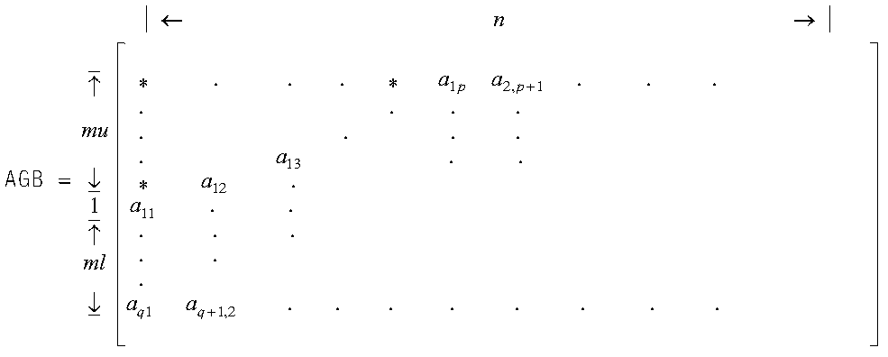
where "*" means you do not store an element in that position in the array. These positions are not accessed by ESSL. Unused positions in the array always occur in the upper left triangle of the array, but may not occur in the lower right triangle of the array, as you can see from the examples given here.
Following is an example where m > n, and general band matrix A is 9 by 8 with band widths of ml = 2 and mu = 3.
Given the following matrix A:
                *                                *
                | 11  12  13  14   0   0   0   0 |
                | 21  22  23  24  25   0   0   0 |
                | 31  32  33  34  35  36   0   0 |
                |  0  42  43  44  45  46  47   0 |
                |  0   0  53  54  55  56  57  58 |
                |  0   0   0  64  65  66  67  68 |
                |  0   0   0   0  75  76  77  78 |
                |  0   0   0   0   0  86  87  88 |
                |  0   0   0   0   0   0  97  98 |
                *                                *
you store it in array AGB, declared as AGB(6,8), as follows, where a11 is stored in AGB(4,1):
                *                                *
                |  *   *   *  14  25  36  47  58 |
                |  *   *  13  24  35  46  57  68 |
         AGB =  |  *  12  23  34  45  56  67  78 |
                | 11  22  33  44  55  66  77  88 |
                | 21  32  43  54  65  76  87  98 |
                | 31  42  53  64  75  86  97   * |
                *                                *
Following is an example where m < n, and general band matrix A is 7 by 9 with band widths of ml = 2 and mu = 3.
Given the following matrix A:
              *                                    *
              | 11  12  13  14   0   0   0   0   0 |
              | 21  22  23  24  25   0   0   0   0 |
              | 31  32  33  34  35  36   0   0   0 |
              |  0  42  43  44  45  46  47   0   0 |
              |  0   0  53  54  55  56  57  58   0 |
              |  0   0   0  64  65  66  67  68  69 |
              |  0   0   0   0  75  76  77  78  79 |
              *                                    *
you store it in array AGB, declared as AGB(6,9), as follows, where a11 is stored in AGB(4,1) and the leading diagonal does not fill up the whole row:
              *                                    *
              |  *   *   *  14  25  36  47  58  69 |
              |  *   *  13  24  35  46  57  68  79 |
        AGB = |  *  12  23  34  45  56  67  78   * |
              | 11  22  33  44  55  66  77   *   * |
              | 21  32  43  54  65  76   *   *   * |
              | 31  42  53  64  75   *   *   *   * |
              *                                    *
and where "*" means you do not store an element in that position in the array.
Following is an example of how to transform your general band matrix, for all values of m and n, to BLAS-general-band storage mode:
        DO 20 J=1,N
           K=MU+1-J
           DO 10 I=MAX(1,J-MU),MIN(M,J+ML)
              AGB(K+I,J)=A(I,J)
   10      CONTINUE
   20   CONTINUE
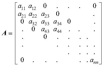
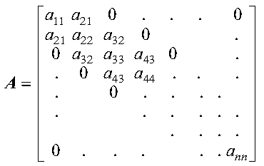
A symmetric band matrix is a symmetric matrix whose nonzero elements are arranged uniformly near the diagonal, such that:
where k is the half band width.
The following matrix illustrates a symmetric band matrix of order n, where the half band width k = q-1:
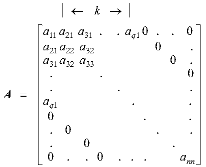
The two storage modes used for storing symmetric band matrices are described in the following sections:
Only the band elements of the upper triangular part of a symmetric band matrix, including the main diagonal, are stored for upper-band-packed storage mode.
For a matrix A of order n and a half band width of k, the array must have a leading dimension, lda, greater than or equal to k+1, and the size of the second dimension must be (at least) n.
Using array ASB, which is declared as ASB(lda,n), where p = lda = k+1, the elements of a symmetric band matrix are stored as follows:
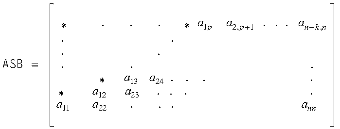
where "*" means you do not store an element in that position in the array.
Following is an example of a symmetric band matrix A of order 6 and a half band width of 3.
Given the following matrix A:
                    *                        *
                    | 11  12  13  14   0   0 |
                    | 12  22  23  24  25   0 |
                    | 13  23  33  34  35  36 |
                    | 14  24  34  44  45  46 |
                    |  0  25  35  45  55  56 |
                    |  0   0  36  46  56  66 |
                    *                        *
you store it in upper-band-packed storage mode in array ASB, declared as ASB(4,6), as follows.
                    *                        *
                    |  *   *   *  14  25  36 |
              ASB = |  *   *  13  24  35  46 |
                    |  *  12  23  34  45  56 |
                    | 11  22  33  44  55  66 |
                    *                        *
Following is an example of how to transform your symmetric band matrix to upper-band-packed storage mode:
      DO 20 J=1,N
         M=K+1-J
         DO 10 I=MAX(1,J-K),J
            ASB(M+I,J)=A(I,J)
      10 CONTINUE
   20 CONTINUE
Only the band elements of the lower triangular part of a symmetric band matrix, including the main diagonal, are stored for lower-band-packed storage mode.
For a matrix A of order n and a half band width of k, the array must have a leading dimension, lda, greater than or equal to k+1, and the size of the second dimension must be (at least) n.
Using array ASB, which is declared as ASB(lda,n), where q = lda = k+1, the elements of a symmetric band matrix are stored as follows:
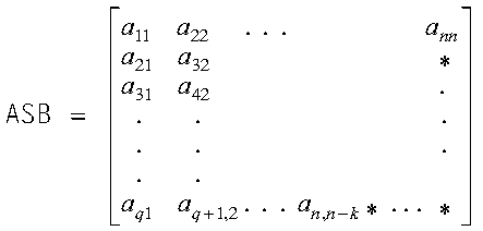
where "*" means you do not store an element in that position in the array.
Following is an example of a symmetric band matrix A of order 6 and a half band width of 2.
Given the following matrix A:
                    *                        *
                    | 11  21  31   0   0   0 |
                    | 21  22  32  42   0   0 |
                    | 31  32  33  43  53   0 |
                    |  0  42  43  44  54  64 |
                    |  0   0  53  54  55  65 |
                    |  0   0   0  64  65  66 |
                    *                        *
you store it in lower-band-packed storage mode in array ASB, declared as ASB(3,6), as follows:
                    *                        *
                    | 11  22  33  44  55  66 |
              ASB = | 21  32  43  54  65   * |
                    | 31  42  53  64   *   * |
                    *                        *
Following is an example of how to transform your symmetric band matrix to lower-band-packed storage mode:
      DO 20 J=1,N
         DO 10 I=J,MIN(J+K,N)
            ASB(I-J+1,J)=A(I,J)
      10 CONTINUE
   20 CONTINUE
A real symmetric band matrix A is positive definite if and only if xTAx is positive for all nonzero vectors x.
The positive definite symmetric band matrix is stored in the same way a symmetric band matrix is stored. For a description of this storage technique, see Symmetric Band Matrix.
A complex band matrix is Hermitian if it is equal to its conjugate transpose:
The complex Hermitian band matrix is stored using the same two techniques used for symmetric band matrices:
Following is an example of a complex Hermitian band matrix H of order 5, having a half band width of 2.
Given the following matrix H:
           *                                              *
           | (11,  0) (21, -1) (31,  1)  (0,  0)  (0,  0) |
           | (21,  1) (22,  0) (32, -1) (42, -1)  (0,  0) |
           | (31, -1) (32,  1) (33,  0) (43, -1) (53, -1) |
           |  (0,  0) (42,  1) (43,  1) (44,  0) (54, -1) |
           |  (0,  0)  (0,  0) (53,  1) (54,  1) (55,  0) |
           *                                              *
you store it in a two-dimensional array HP, as follows:
          *                                           *
          | (11,  *) (22, *) (33, *) (44,  *) (55, *) |
     HP = | (21,  1) (32, 1) (43, 1) (54,  1)    *    |
          | (31, -1) (42, 1) (53, 1)    *        *    |
          *                                           *
          *                                              *
          |    *        *     (31,  1) (42, -1) (53, -1) |
    HP =  |    *     (21, -1) (32, -1) (43, -1) (54, -1) |
          | (11, *)  (22,  *) (33,  *) (44,  *) (55,  *) |
          *                                              *
where "*" means you do not have to store a value in that position in the array. The imaginary parts of the diagonal elements of a complex Hermitian band matrix are always 0, so you do not need to set these values. The ESSL subroutines always assume that the values in these positions are 0.
There are two types of triangular band matrices: upper triangular band matrix and lower triangular band matrix. Triangular band matrices have the same number of rows as they have columns; that is, they have n rows and n columns. They have an upper or lower band width of k.
A band matrix U is an upper triangular band matrix if its nonzero elements are found only in the upper triangle of the matrix, including the main diagonal; that is:
Its band elements are arranged uniformly near the diagonal in the upper triangle of the matrix, such that:
The following matrix U illustrates an upper triangular band matrix of order n with an upper band width k = q-1:
A band matrix L is a lower triangular band matrix if its nonzero elements are found only in the lower triangle of the matrix, including the main diagonal; that is:
Its band elements are arranged uniformly near the diagonal in the lower triangle of the matrix such that:
The following matrix L illustrates an upper triangular band matrix of order n with a lower band width k = q-1:
A triangular band matrix can also be a unit triangular band matrix if all the diagonal elements have a value of 1. For an illustration of a unit triangular matrix, see Triangular Matrix.
The two storage modes used for storing triangular band matrices are described in the following sections:
It is important to note that because the diagonal elements of a unit triangular band matrix are always one, you do not need to set these values in the array for these two storage modes. ESSL always assumes that the values in these positions are one.
Only the band elements of the upper triangular part of an upper triangular band matrix, including the main diagonal, are stored for upper-triangular-band-packed storage mode.
For a matrix U of order n and an upper band width of k, the array must have a leading dimension, lda, greater than or equal to k+1, and the size of the second dimension must be (at least) n.
Using array UTB, which is declared as UTB(lda,n), where p = lda = k+1, the elements of an upper triangular band matrix are stored as follows:
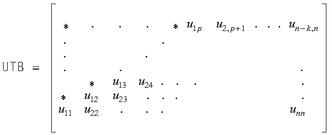
where "*" means you do not store an element in that position in the array.
Following is an example of an upper triangular band matrix U of order 6 and an upper band width of 3.
Given the following matrix U:
                    *                        *
                    | 11  12  13  14   0   0 |
                    |  0  22  23  24  25   0 |
                    |  0   0  33  34  35  36 |
                    |  0   0   0  44  45  46 |
                    |  0   0   0   0  55  56 |
                    |  0   0   0   0   0  66 |
                    *                        *
you store it in upper-triangular-band-packed storage mode in array UTB, declared as UTB(4,6), as follows:
                    *                        *
                    |  *   *   *  14  25  36 |
             UTB =  |  *   *  13  24  35  46 |
                    |  *  12  23  34  45  56 |
                    | 11  22  33  44  55  66 |
                    *                        *
Following is an example of how to transform your upper triangular band matrix to upper-triangular-band-packed storage mode:
      DO 20 J=1,N
         M=K+1-J
         DO 10 I=MAX(1,J-K),J
            UTB(M+I,J)=U(I,J)
      10 CONTINUE
   20 CONTINUE
Only the band elements of the lower triangular part of a lower triangular band matrix, including the main diagonal, are stored for lower-triangular-band-packed storage mode.
For a matrix L of order n and a lower band width of k, the array must have a leading dimension, lda, greater than or equal to k+1, and the size of the second dimension must be (at least) n.
Using array LTB, which is declared as LTB(lda,n), where q = lda = k+1, the elements of a lower triangular band matrix are stored as follows:
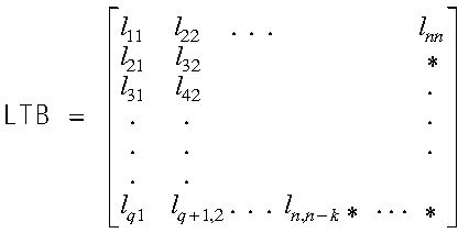
where "*" means you do not store an element in that position in the array.
Following is an example of a lower triangular band matrix L of order 6 and a lower band width of 2.
Given the following matrix L:
                    *                        *
                    | 11   0   0   0   0   0 |
                    | 21  22   0   0   0   0 |
                    | 31  32  33   0   0   0 |
                    |  0  42  43  44   0   0 |
                    |  0   0  53  54  55   0 |
                    |  0   0   0  64  65  66 |
                    *                        *
you store it in lower-triangular-band-packed storage mode in array LTB, declared as LTB(3,6), as follows:
                    *                        *
                    | 11  22  33  44  55  66 |
             LTB =  | 21  32  43  54  65   * |
                    | 31  42  53  64   *   * |
                    *                        *
Following is an example of how to transform your lower triangular band matrix to lower-triangular-band-packed storage mode:
      DO 20 J=1,N
         M=1-J
         DO 10 I=J,MIN(N,J+K)
            LTB(M+I,J)=L(I,J)
      10 CONTINUE
   20 CONTINUE
A general tridiagonal matrix is a matrix whose nonzero elements are found only on the diagonal, subdiagonal, and superdiagonal of the matrix; that is:
The following matrix illustrates a general tridiagonal matrix of order n:
Only the diagonal, subdiagonal, and superdiagonal elements of the general tridiagonal matrix are stored. This is called tridiagonal storage mode. The elements of a general tridiagonal matrix, A, of order n are stored in three one-dimensional arrays, C, D, and E, each of length n, where array C contains the subdiagonal elements, stored as follows:
and array D contains the main diagonal elements, stored as follows:
and array E contains the superdiagonal elements, stored as follows:
where "*" means you do not store an element in that position in the array.
Following is an example of a general tridiagonal matrix A of order 5:
                      *                    *
                      | 11  12   0   0   0 |
                      | 21  22  23   0   0 |
                      |  0  32  33  34   0 |
                      |  0   0  43  44  45 |
                      |  0   0   0  54  55 |
                      *                    *
which you store in tridiagonal storage mode in arrays C, D, and E, each of length 5, as follows:
                       C = (*, 21, 32, 43, 54)

                       D = (11, 22, 33, 44, 55)

                       E = (12, 23, 34, 45, *)
A tridiagonal matrix A is also symmetric if and only if its nonzero elements are found only on the diagonal, subdiagonal, and superdiagonal of the matrix, and its subdiagonal elements and superdiagonal elements are equal; that is:
The following matrix illustrates a symmetric tridiagonal matrix of order n:
Only the diagonal and subdiagonal elements of the positive definite symmetric tridiagonal matrix are stored. This is called symmetric-tridiagonal storage mode. The elements of a symmetric tridiagonal matrix A of order n are stored in two one-dimensional arrays C and D, each of length n, where array C contains the subdiagonal elements, stored as follows:
where "*" means you do not store an element in that position in the array. Then array D contains the main diagonal elements,stored as follows:
Following is an example of a symmetric tridiagonal matrix A of order 5:
                      *                    *
                      | 10   1   0   0   0 |
                      |  1  20   2   0   0 |
                      |  0   2  30   3   0 |
                      |  0   0   3  40   4 |
                      |  0   0   0   4  50 |
                      *                    *
which you store in symmetric-tridiagonal storage mode in arrays C and D, each of length 5, as follows:
                       C = (*, 1, 2, 3, 4)

                       D = (10, 20, 30, 40, 50)
A real symmetric tridiagonal matrix A is positive definite if and only if xTAx is positive for all nonzero vectors x.
The positive definite symmetric tridiagonal matrix is stored in the same way the symmetric tridiagonal matrix is stored. For a description of this storage technique, see Symmetric Tridiagonal Matrix.
A sparse matrix is a matrix having a relatively small number of nonzero elements.
Consider the following as an example of a sparse matrix A:
                    *                        *
                    | 11   0  13   0   0   0 |
                    | 21  22   0  24   0   0 |
                    |  0  32  33   0  35   0 |
                    |  0   0  43  44   0  46 |
                    | 51   0   0  54  55   0 |
                    | 61  62   0   0  65  66 |
                    *                        *
A sparse matrix can be stored in full-matrix storage mode or a packed storage mode. When a sparse matrix is stored in full-matrix storage mode, all its elements, including its zero elements, are stored in an array.
The seven packed storage modes used for storing sparse matrices are described in the following sections:
The sparse matrix A, stored in compressed-matrix storage mode, uses two two-dimensional arrays to define the sparse matrix storage, AC and KA. See reference [73]. Given the m by n sparse matrix A, having a maximum of nz nonzero elements in each row:
Unless all the rows of sparse matrix A contain approximately the same number of nonzero elements, this storage mode requires a large amount of storage. This diminishes the performance you can obtain by using this storage mode.
Consider the following as an example of a 6 by 6 sparse matrix A with a maximum of four nonzero elements in each row. It shows how matrix A can be stored in arrays AC and KA.
Given the following matrix A:
                    *                        *
                    | 11   0  13   0   0   0 |
                    | 21  22   0  24   0   0 |
                    |  0  32  33   0  35   0 |
                    |  0   0  43  44   0  46 |
                    | 51   0   0  54  55   0 |
                    | 61  62   0   0  65  66 |
                    *                        *
the arrays are:
                        *                *
                        | 11  13   0   0 |
                        | 22  21  24   0 |
                  AC =  | 33  32  35   0 |
                        | 44  43  46   0 |
                        | 55  51  54   0 |
                        | 66  61  62  65 |
                        *                *
                          *            *
                          | 1  3  *  * |
                          | 2  1  4  * |
                    KA =  | 3  2  5  * |
                          | 4  3  6  * |
                          | 5  1  4  * |
                          | 6  1  2  5 |
                          *            *
where "*" means you can store any value from 1 to 6 in that position in the array.
Symmetric sparse matrices use the same storage technique as nonsymmetric sparse matrices; that is, all nonzero elements of a symmetric matrix A must be stored in array AC, not just the elements of the upper triangle and diagonal of matrix A.
In general terms, this storage technique can be expressed as follows:
where:
The storage mode used for square sparse matrices stored in compressed-diagonal storage mode has two variations, depending on whether the matrix is a general sparse matrix or a symmetric sparse matrix. This section explains both of these variations. This section begins, however, by explaining the conventions used for numbering the diagonals in the matrix, which apply to the storage descriptions.
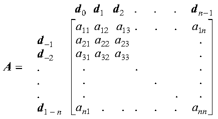
Matrix A of order n has 2n-1 diagonals. Because k = j-i is constant for the elements aij along each diagonal, each diagonal can be assigned a diagonal number, k, having a value from 1-n to n-1. Then the diagonals can be referred to as dk, where k = 1-n, n-1.
The following matrix shows the starting position of each diagonal, dk:
For a general (square) sparse matrix A, compressed-diagonal storage mode uses two arrays to define the sparse matrix storage, AD and LA. Using the above convention for numbering the diagonals, and given that sparse matrix A contains nd diagonals having nonzero elements, arrays AD and LA are set up as follows:
The diagonals can be stored in any columns in array AD.
Because this storage mode requires entire diagonals to be stored, if the nonzero elements in matrix A are not concentrated along a few diagonals, this storage mode requires a large amount of storage. This diminishes the performance you obtain by using this storage mode.
Consider the following as an example of how a 6 by 6 general sparse matrix A with 5 nonzero diagonals is stored in arrays AD and LA.
Given the following matrix A:
                    *                        *
                    | 11   0  13   0   0   0 |
                    | 21  22   0  24   0   0 |
                    |  0  32  33   0  35   0 |
                    |  0   0  43  44   0  46 |
                    | 51   0   0  54  55   0 |
                    | 61  62   0   0  65  66 |
                    *                        *
the arrays are:
                          *                    *
                          | 11  13   0   0   0 |
                          | 22  24  21   0   0 |
                  AD   =  | 33  35  32   0   0 |
                          | 44  46  43   0   0 |
                          | 55   0  54  51   0 |
                          | 66   0  65  62  61 |
                          *                    *

                  LA   =  (0, 2, -1, -4, -5)
For a symmetric sparse matrix, where each superdiagonal k is equal to subdiagonal -k, compressed-diagonal storage mode uses the same storage technique as for the general sparse matrix, except that only the nonzero main diagonal and one diagonal of each couple of nonzero diagonals, k and -k, are used in setting up arrays AD and LA. You can store either the upper or the lower diagonal of each couple.
Consider the following as an example of a symmetric sparse matrix of order 6 and how it is stored in arrays AD and LA, using only three nonzero diagonals in the matrix.
Given the following matrix A:
                    *                        *
                    | 11   0  13   0  51   0 |
                    |  0  22   0  24   0  62 |
                    | 13   0  33   0  35   0 |
                    |  0  24   0  44   0  46 |
                    | 51   0  35   0  55   0 |
                    |  0  62   0  46   0  66 |
                    *                        *
the arrays are:
                             *            *
                             | 11  13   0 |
                             | 22  24   0 |
                     AD   =  | 33  35   0 |
                             | 44  46   0 |
                             | 55   0  51 |
                             | 66   0  62 |
                             *            *

                      LA   = (0, 2, -4)
In general terms, this storage technique can be expressed as follows:
where:
For a sparse matrix A, storage-by-indices uses three one-dimensional arrays to define the sparse matrix storage, AR, IA, and JA. Given the m by n sparse matrix A having ne nonzero elements, the arrays are set up as follows:
Consider the following as an example of a 6 by 6 sparse matrix A and how it can be stored in arrays AR, IA, and JA.:
Given the following matrix A:
                    *                        *
                    | 11   0  13   0   0   0 |
                    | 21  22   0  24   0   0 |
                    |  0  32  33   0  35   0 |
                    |  0   0  43  44   0  46 |
                    |  0   0   0   0   0   0 |
                    | 61  62   0   0  65  66 |
                    *                        *
the arrays are:
    AR = (11, 22, 32, 33, 13, 21, 43, 24, 66, 46, 35, 62, 61, 65, 44)

    IA = (1, 2, 3, 3, 1, 2, 4, 2, 6, 4, 3, 6, 6, 6, 4)

    JA = (1, 2, 2, 3, 3, 1, 3, 4, 6, 6, 5, 2, 1, 5, 4)
In general terms, this storage technique can be expressed as follows:
where:
For a sparse matrix, A, storage-by-columns uses three one-dimensional arrays to define the sparse matrix storage, AR, IA, and JA. Given the m by n sparse matrix A having ne nonzero elements, the arrays are set up as follows:
Consider the following as an example of a 6 by 6 sparse matrix A and how it can be stored in arrays AR, IA, and JA.
Given the following matrix A:
                    *                       *
                    | 11   0  13   0  0   0 |
                    | 21  22   0  24  0   0 |
                    |  0  32  33   0  0   0 |
                    |  0   0  43  44  0  46 |
                    |  0   0   0   0  0   0 |
                    | 61  62   0   0  0  66 |
                    *                       *
the arrays are:
    AR = (11, 61, 21, 62, 32, 22, 13, 33, 43, 44, 24, 46, 66)

    IA = (1, 6, 2, 6, 3, 2, 1, 3, 4, 4, 2, 4, 6)

    JA = (1, 4, 7, 10, 12, 12, 14)
In general terms, this storage technique can be expressed as follows:
where:
The storage mode used for sparse matrices stored by rows has three variations, depending on whether the matrix is a general sparse matrix or a symmetric sparse matrix. This section explains these variations.
For a general sparse matrix A, storage-by-rows uses three one-dimensional arrays to define the sparse matrix storage, AR, IA, and JA. Given the m by n sparse matrix A having ne nonzero elements, the arrays are set up as follows:
Consider the following as an example of a 6 by 6 general sparse matrix A and how it can be stored in arrays AR, IA, and JA.
Given the following matrix A:
                    *                       *
                    | 11   0  13   0  0   0 |
                    | 21  22   0  24  0   0 |
                    |  0  32  33   0  0   0 |
                    |  0   0  43  44  0  46 |
                    |  0   0   0   0  0   0 |
                    | 61  62   0   0  0  66 |
                    *                       *
the arrays are:
    AR = (11, 13, 24, 22, 21, 32, 33, 44, 43, 46, 61, 62, 66)

    IA = (1, 3, 6, 8, 11, 11, 14)

    JA = (1, 3, 4, 2, 1, 2, 3, 4, 3, 6, 1, 2, 6)
For a symmetric sparse matrix of order m, storage-by-rows uses the same storage technique as for the general sparse matrix, except that only the upper or lower triangle and diagonal elements are used in setting up arrays AR, IA, and JA.
Consider the following as an example of a symmetric sparse matrix A of order 6 and how it can be stored in arrays AR, IA, and JA using upper-storage-by-rows, which stores only the upper triangle and diagonal elements.
Given the following matrix A:
                    *                        *
                    | 11   0  13   0   0   0 |
                    |  0  22  23  24   0   0 |
                    | 13  23  33   0  35   0 |
                    |  0  24   0  44   0  46 |
                    |  0   0  35   0  55   0 |
                    |  0   0   0  46   0   0 |
                    *                        *
the arrays are:
    AR = (11, 13, 22, 24, 23, 33, 35, 46, 44, 55)

    IA = (1, 3, 6, 8, 10, 11, 11)

    JA = (1, 3, 2, 3, 4, 3, 5, 4, 6, 5)
Using the same symmetric matrix A, consider the following as an example of how it can be stored in arrays AR, IA, and JA using lower-storage-by-rows, which stores only the lower triangle and diagonal elements:
    AR = (11, 22, 23, 33, 13, 24, 44, 55, 35, 46)

    IA = (1, 2, 3, 6, 8, 10, 11 )

    JA = (1, 2, 2, 3, 1, 2, 4, 5, 3, 4)
In general terms, this storage technique can be expressed as follows:
where:
The diagonal-out skyline storage mode used for sparse matrices has two variations, depending on whether the matrix is a general sparse matrix or a symmetric sparse matrix. Both of these variations are explained here.
For a general sparse matrix A, diagonal-out skyline storage mode uses four one-dimensional arrays to define the sparse matrix storage, AU, IDU, AL, and IDL. Given the sparse matrix A of order n, containing nu+nl-n elements under the top and left profiles, the arrays are set up as follows:
Consider the following as an example of a 6 by 6 general sparse matrix A and how it is stored in arrays AU, IDU, AL, and IDL.
Given the following matrix A:
                    *                        *
                    |  0  12  13   0   0   0 |
                    | 21  22   0  24   0   0 |
                    | 31   0  33  34   0  36 |
                    | 41  42  43  44  45   0 |
                    |  0   0   0  54  55  56 |
                    |  0   0  63   0  65  66 |
                    *                        *
the arrays are:
AU = (0, 22, 12, 33, 0, 13, 44, 34, 24, 55, 45, 66, 56, 0, 36)
IDU = (1, 2, 4, 7, 10, 12, 16) where nu=15
AL = (*, *, 21, *, 0, 31, *, 43, 42, 41, *, 54, *, 65, 0, 63)
IDL = (1, 2, 4, 7, 11, 13, 17) where nl=16
and where "*" means you do not have to store a value in that position in the array. However, these storage positions are required.
For a symmetric sparse matrix of order n, diagonal-out skyline storage mode uses the same storage technique as for the upper triangle and diagonal elements of the general sparse matrix; therefore, only the AU and IDU arrays are needed.
Consider the following as an example of a symmetric sparse matrix A of order 6 and how it is stored in arrays AU and IDU.
Given the following matrix A:
                    *                        *
                    |  0  12  13   0   0   0 |
                    | 12  22   0  24   0   0 |
                    | 13   0  33  34   0  36 |
                    |  0  24  34  44  45   0 |
                    |  0   0   0  45  55  56 |
                    |  0   0  36   0  56  66 |
                    *                        *
the arrays are:
AU = (0, 22, 12, 33, 0, 13, 44, 34, 24, 55, 45, 66, 56, 0, 36)
IDU = (1, 2, 4, 7, 10, 12, 16) where nu=15
In general terms, this storage technique can be expressed as follows:
where:
The profile-in skyline storage mode used for sparse matrices has two variations, depending on whether the matrix is a general sparse matrix or a symmetric sparse matrix. Both of these variations are explained here.
For a general sparse matrix A, profile-in skyline storage mode uses four one-dimensional arrays to define the sparse matrix storage, AU, IDU, AL, and IDL. Given the sparse matrix A of order n, containing nu+nl-n elements under the top and left profiles, the arrays are set up as follows:
Consider the following as an example of a 6 by 6 general sparse matrix A and how it is stored in arrays AU, IDU, AL, and IDL.
Given the following matrix A:
                    *                        *
                    |  0  12  13   0   0   0 |
                    | 21  22   0  24   0   0 |
                    | 31   0  33  34   0  36 |
                    | 41  42  43  44  45   0 |
                    |  0   0   0  54  55  56 |
                    |  0   0  63   0  65  66 |
                    *                        *
the arrays are:
AU = (0, 12, 22, 13, 0, 33, 24, 34, 44, 45, 55, 36, 0, 56, 66)
IDU = (1, 3, 6, 9, 11, 15, 16) where nu=15
AL = (*, 21, *, 31, 0, *, 41, 42, 43, *, 54, *, 63, 0, 65, *)
IDL = (1, 3, 6, 10, 12, 16, 17) where nl=16
and where "*" means you do not have to store a value in that position in the array. However, these storage positions are required.
For a symmetric sparse matrix of order n, profile-in skyline storage mode uses the same storage technique as for the upper triangle and diagonal elements of the general sparse matrix; therefore, only the AU and IDU arrays are needed.
Consider the following as an example of a symmetric sparse matrix A of order 6 and how it is stored in arrays AU and IDU.
Given the following matrix A:
                    *                        *
                    |  0  12  13   0   0   0 |
                    | 12  22   0  24   0   0 |
                    | 13   0  33  34   0  36 |
                    |  0  24  34  44  45   0 |
                    |  0   0   0  45  55  56 |
                    |  0   0  36   0  56  66 |
                    *                        *
the arrays are:
AU = (0, 12, 22, 13, 0, 33, 24, 34, 44, 45, 55, 36, 0, 56, 66)
IDU = (1, 3, 6, 9, 11, 15, 16) where nu=15
In general terms, this storage technique can be expressed as follows:
where: